 |
| |||||
| Protein Homology/analogY Recognition Engine V 2.0 | ||||||
|
|
|
| |||||
| Protein Homology/analogY Recognition Engine V 2.0 | ||||||
|
Interpreting Results: Normal |
|
1. Overview/pipeline 1. Overview/pipeline'Normal' mode modelling by Phyre2 produces a set of potential 3D models of your protein based on alignment to known protein structures. The pipeline involves:
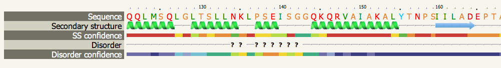
Secondary structure and disorder predictionBelow is a snippet of a typical prediction. The position in the sequence is indicated in the top line. The sequence is represented on the next line with residues coloured according to a simple property-based scheme:
There is no magic recipe to colour amino acid types, but this is a scheme I have found useful in the past. If anyone feels particularly strongly about this please let me know and I can adjust the colour scheme.
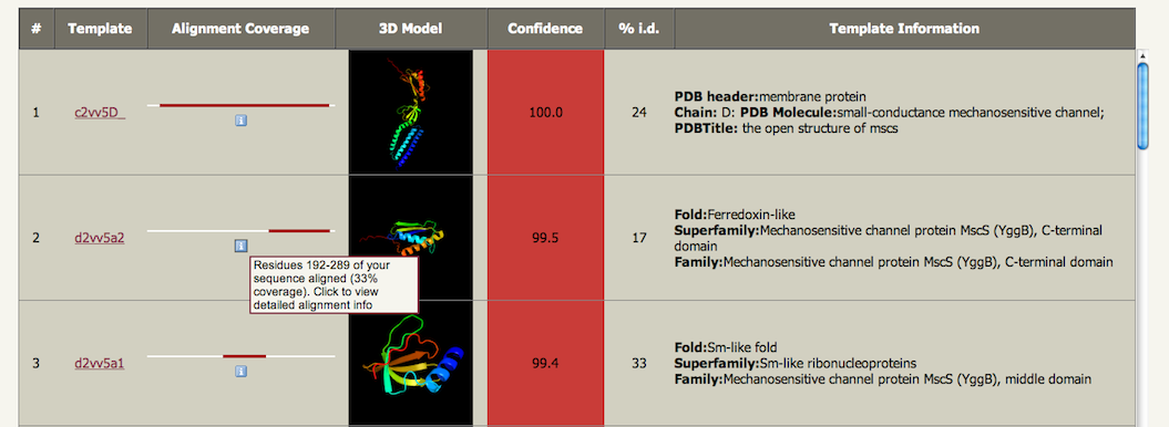
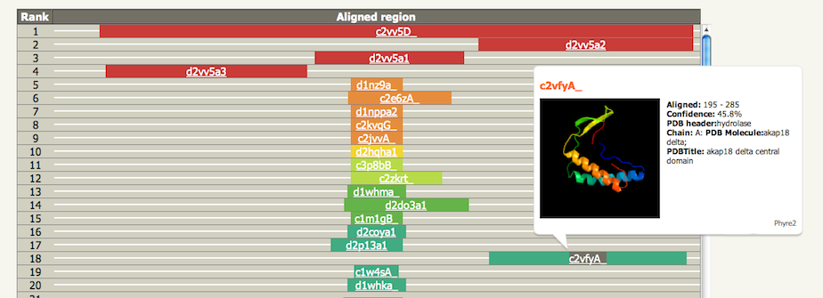
The prediction is 3-state: either α-helix, β-strand or coil. Green helices represent α-helices, blue arrows indicate β-strands and faint lines indicate coil. The 'SS confidence' line indicates the confidence in the prediction, with red being high confidence and blue low confidence. You can see in this example that the 1st and 4th helices are predicted with high confidence as is the strand at the end. However the two middle helices are associated with orange, yellow and green indicating a weak prediction. The 'Disorder' line contains the prediction of disordered regions in your protein and such regions are indicated by question marks (?). As you can see, the weakest region of helix prediction coincides with a relatively strong prediction of disorder. Disordered regions can often by functionally very important. However, because they are disordered, there is not much point trying to predict their structure! Secondary structure and disorder prediction is on average 78-80% accurate (i.e. 78-80% of the residues are predicted to be in their correct state). However, this accuracy is only reached if there is a substantial number of diverse sequence homologues detectable in the sequence database. If your sequence has very few homologues (something you can check by looking at the PSI-Blast results via the button near the top of the results page) then accuracy falls to approximately 65%. Also we are not predicting β-turns, β-bends π-helices, or 310-helices. These classes are merged together so that β-turns and β-bends are treated as coil, and π-helices and 310-helices are considered α-helices. Domain analysisThe domain analysis section illustrates where along your sequence matches have been found, colour-coded by confidence. In the example below you can see that this protein appears to be composed of 3 domains. The top red line indicates a confident (red) match to the entire length of the protein to fold library entry c2vv5D_. The initial 'c' indicates this protein is a whole chain taken from the PDB, with PDB identifier 2vv5 and chain identifier D. The next three red lines each cover a different portion of the sequence and have codes d2vv5a1, d2vv5a2 and d2vv5a3. These codes are from SCOP as indicated by the initial 'd' standing for domain. These are three domains from PDB identifier 2vv5 chain A. Below these hits we start to see the colours changing to oranges and green indicating a drop in confidence of the match. If you hover over one of the codes a pop-up summary is displayed showing the model and information about the template used. Further down the list (not shown here) will be coloured-lines but no links. These are matches detected but not modelled by Phyre2. |
 |
Detailed template information (and models)This section contains the really important stuff - the models! The matches are ranked by a raw alignment score (not shown) that is
based on the number of aligned residues and the quality of
alignment. This in turn is based on the similarity of residue
probability distributions for each position, secondary structure
similarity and the presence or absence of insertions and deletions. Each row provides information
on the template used for the model and a small graphic indicating where
along your sequence is the match colour-coded by confidence. Beneath
that line graphic is an info icon The image is a picture of the model constructed for your sequence based on that template. Clicking on the picture will download the coordinates of the model in PDB format for input to any other viewing or analysis programs you may have. The next column is 'Confidence'. This represents the probability (from 0 to 100) that the match between your sequence and this template is a true homology. It DOES NOT represent the expected accuracy of the model - although the two are intimately related. I will be including an analysis of model accuracy soon, but such techniques are still quite unreliable. If you have a match with confidence >90%, one can generally be very confident that your protein adopts the overall fold shown and that the core of the protein is modelled at high accuracy (2-4Å rmsd from native,true structure). However, surface loops will probably deviate from the native.
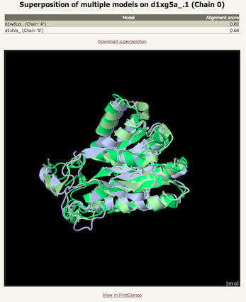
This brings us to the next important piece of information in determining the likely accuracy of the model: the percentage identity between your sequence and the template. For extremely high accuracy models you want this number to be above 30-40%. However it is important to understand that even at very low sequence identities (<15%) models can be very useful as long as the confidence is high. Finally, the last column provides information on the template taken either from SCOP or the PDB file itself. This information is very useful for gleaning information about the potential function of your protein. In a later release I will include Gene Ontology (GO) terms for each match to further aid functional annotation. Once again though, transferring specfici functional annotation when two proteins share low sequence identity is error-prone. However, the more general the GO terms, the more confident you can be in transferring the annotation. SuperpositionsAt the bottom of the main table is a button entitled "Generate superposition of selected models". Beneath each template name (column 2) of the main table are two buttons. The one on the left like this: is a radio button allowing you to select one single master model. To its right is a tick box like this: . You can tick as many of these as you wish. Click on the main button below the table and the ticked templates will be superposed on the master model. This will then take you to a page with a large JMol window displaying the superposition for interactive viewing. This can be helpful to establish which regions of the models agree and disagree which in turn can give you a sense for which regions of the model are trustworthy and which regions you should be cautious about.
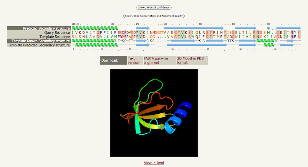
AlignmentEach model built by Phyre2 is based on an alignment generated by
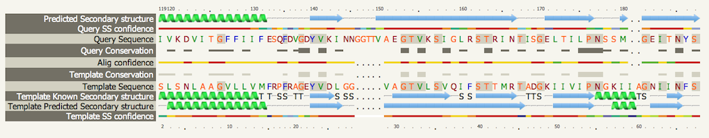
HMM-HMM matching. Clicking on the info icon An example is shown below. Please see the Secondary structure and disorder section for details on basic interpretation. An extra row is present here entitled "Template known secondary structure". Both the predicted secondary structure of your sequence and the known AND predicted secondary structure of the template are used in conjunction with the sequence information in generating the alignment.
In the "Template known secondary structure" section you will also see 'S' and 'T' characters. Sometimes you may also see G,I and B characters. These are assigned secondary structure types by the program DSSP. They represent the following:
Identical residues in the alignment are highlighted with a grey background There are links below the alignment to permit downloading of a text version of the alignment, a simple pairwise representation of the alignment in FASTA format and a link to the coordinates of the model in PDB format. Beneath the image of the model is a link that launches the JMol java applet inside the browser to interactively inspect the model. At the top of the screen are two buttons that can add/remove detail from the alignment. If you click both buttons the result can be seen below
The 'Conservation' rows contain information on residue conservation across the detected sequence homologues classed into 3 states. No symbol indicates unconserved, a thin grey bar indicates moderate conservation and a large block indicates a high degree of conservation. Confidence lines are explained in the Secondary structure and disorder section. Transmembrane helix predictionYour sequence and the set of homologues detected by PSI-Blast are processed by a Support Vector Machine (a powerful machine learning tool) to a) determine whether your sequence is likely to contain transmembrane helices and b) predict their topology in the membrane. For this Phyre2 uses memsat-svm which has demonstrated an average accuracy of 89% on a large test set. An example image is shown below. The extracellular and cytoplasmic sides of the membrane are labelled and the beginning and end of each transmembrane helix illustrated with a number indicating the residue index. |
|
|
Phyre is now FREE for commercial users!
All images and data generated by Phyre2 are free to use in any publication with acknowledgement
Accessibility Statement| Please cite: Phyre2.2: A Community Resource for Template-based Protein Structure Prediction | |||||||||
| Powell HR et al. Journal of Molecular Biology (2025) in press DOI: https://doi.org/10.1016/j.jmb.2025.168960 | |||||||||
|
|
||||||||
 . Hovering over that icon gives you some
numbers about the position and percentage of the alignment. Clicking
it will take you to detailed
. Hovering over that icon gives you some
numbers about the position and percentage of the alignment. Clicking
it will take you to detailed