Hungarian Method |
 |
PHUNKEEPairing subgrapHs Using NetworK Environment Equivalence |
Hungarian Method |
 |
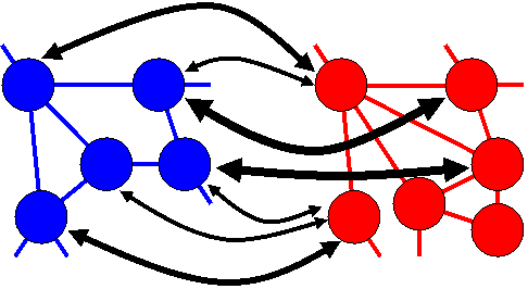
| The Hungarian method was used to reduce the many-to-many sequence similarity relationships between proteins in the two networks to the optimal one-to-one node matching. For each possible protein matching a score based on the logarithm of the BLAST E-value is allocated. The Hungarian method locates the set of one-to-one node matches that optimise the overall score in a manner similar to that of the example shown below. | |
A worked example | |
| To demonstrate how the Hungarian method works, we consider a simple example in which we want to find the optimum match between four Blue nodes and four Red nodes. The score for each potential match is shown in the table below. A lower score indicates a more favourable match, so we want to find a set of node matches that minimises the overall score. |
| Red1 | Red2 | Red3 | Red4 | ||
|---|---|---|---|---|---|
| Blue1 | 8 | 17 | 3 | 23 | |
| Blue2 | 39 | 4 | 11 | 20 | |
| Blue3 | 13 | 2 | 41 | 6 | |
| Blue4 | 22 | 8 | 9 | 2 | |
Step 1First for each row we subtract the row minimum from the rest of the row. |
| Red1 | Red2 | Red3 | Red4 | ||
|---|---|---|---|---|---|
| Blue1 | 8 | 17 | 3 | 23 | -3 |
| Blue2 | 39 | 4 | 11 | 20 | -4 |
| Blue3 | 13 | 2 | 41 | 6 | -2 |
| Blue4 | 22 | 8 | 9 | 2 | -2 |
Step 2Then for each column we subtract the column minimum from the rest of the column. |
| Red1 | Red2 | Red3 | Red4 | ||
|---|---|---|---|---|---|
| Blue1 | 5 | 14 | 0 | 20 | |
| Blue2 | 35 | 0 | 7 | 16 | |
| Blue3 | 11 | 0 | 39 | 4 | |
| Blue4 | 20 | 6 | 7 | 0 | |
| -5 | -0 | -0 | -0 |
Step 3Cover the minimum number of rows or columns required to cover all of the zeros in the matrix (shown in light green). If the number of rows or columns required is equal to the number of rows/columns in the matrix then we are finished. Otherwise, we have to proceed to the next step. In this case, we can cover all zeroes with only three lines so we continue. |
| Red1 | Red2 | Red3 | Red4 | ||
|---|---|---|---|---|---|
| Blue1 | 0 | 14 | 0 | 20 | |
| Blue2 | 30 | 0 | 7 | 16 | |
| Blue3 | 6 | 0 | 39 | 4 | |
| Blue4 | 15 | 6 | 7 | 0 | |
Step 4From the above matrix, we first have to find the minimum value not covered (Blue3-Red1 - 6). This value is then subtracted from each uncovered entry and added to each entry covered by both a vertical and horizontal line (Blue1-Red2 and Blue1-Red4) to give the matrix shown below. Step 3 is then repeated. This continues until four rows or columns are needed to cover all zeroes and we are finished. In this case, the matrix shown below is finished. The zeroes in the matrix determine the optimal matching between nodes. The only possible matching is shown by the zeroes in the purple cells. The final node matches are listed below. |
| Red1 | Red2 | Red3 | Red4 | ||
|---|---|---|---|---|---|
| Blue1 | 0 | 20 | 0 | 26 | |
| Blue2 | 24 | 0 | 1 | 16 | |
| Blue3 | 0 | 0 | 33 | 4 | |
| Blue4 | 9 | 6 | 1 | 0 | |
Node matching assignments
Blue1 = Red3 | |
| Contact Structural Bioinformatics Group Division of Molecular Biosciences Imperial College, London |
  |