Secondary Structure Prediction methods and links
There are now many web servers for structure prediction, here is quick summary:
- PSI-pred (PSI-BLAST profiles used for prediction; David Jones, Warwick)
- JPRED Consensus prediction (includes many of the methods given below; Cuff & Barton, EBI)
- DSC King & Sternberg (this server)
- PREDATORFrischman & Argos (EMBL)
- PHD home page Rost & Sander, EMBL, Germany
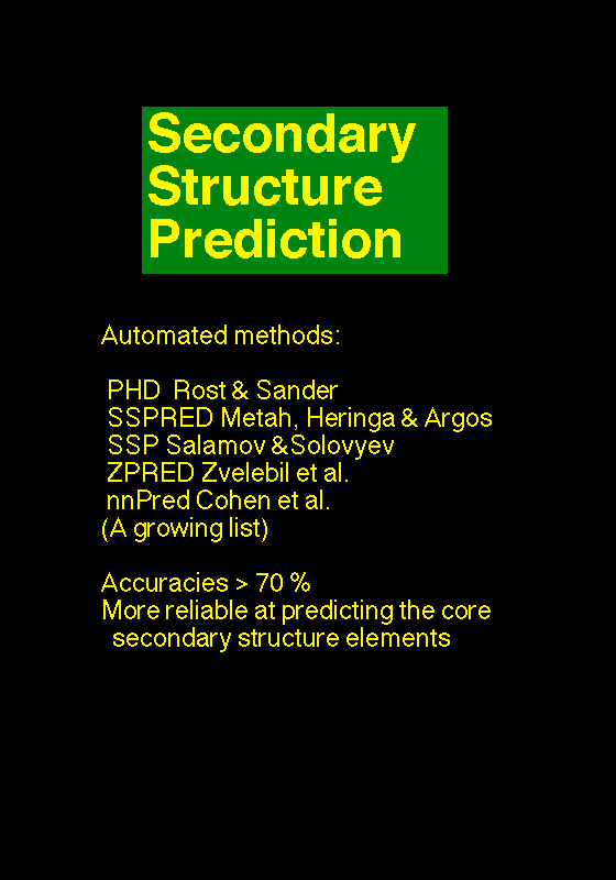
- ZPRED server Zvelebil et al., Ludwig, U.K.
- nnPredict Cohen et al., UCSF, USA.
- BMERC PSA Server Boston University, USA
- SSP (Nearest-neighbor) Solovyev and Salamov, Baylor College, USA.
With no homologue of known structure from which to make a 3D model, a logical next step is to predict
secondary structure. Although they differ in method, the aim of secondary structure prediction is to
provide the location of alpha helices, and beta strands within a protein or protein family.
Methods for single sequences
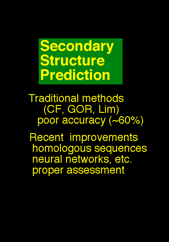
Secondary structure prediction has been around for almost a quarter of a century. The early methods
suffered from a lack of data. Predictions were performed on single sequences rather than families of
homologous sequences, and there were relatively few known 3D structures from which to derive
parameters. Probably the most famous early methods
are those of Chou & Fasman, Garnier, Osguthorbe & Robson (GOR) and Lim. Although the authors
originally claimed quite high accuracies (70-80 %), under careful examination, the methods
were shown to be only between 56 and 60% accurate (see Kabsch & Sander, 1984 given below).
An early problem in secondary structure prediction
had been the inclusion of structures used to derive parameters in the set of structures used
to assess the accuracy of the method.
Some good references on the subject:
- Early methods on single sequences
- Chou, P.Y. & Fasman, G.D. (1974). Biochemistry, 13, 211-222.
- Lim, V.I. (1974). Journal of Molecular Biology, 88, 857-872.
- Garnier, J., Osguthorpe, D.~J. \& Robson, B. (1978).Journal of Molecular Biology, 120, 97-120.
- Kabsch, W. & Sander, C. (1983). FEBS Letters, 155, 179-182. (An assessment of the above methods)
- Later methods on single sequences
- Deleage, G. & Roux, B. (1987). Protein Engineering , 1, 289-294 (DPM)
- Presnell, S.R., Cohen, B.I. & Cohen, F.E. (1992). Biochemistry, 31, 983-993.
- Holley, H.L. & Karplus, M. (1989). Proceedings of the National Academy of Science, 86, 152-156.
- King, R. & Sternberg, M. J.E. (1990). Journal of Molecular Biology, 216, 441-457.
- D. G. Kneller, F. E. Cohen & R. Langridge (1990) Improvements in Protein Secondary Structure Prediction by an Enhanced Neural Network, Journal of Molecular Biology, 214, 171-182. (NNPRED)
Recent improvments
The availability of large families of homologous sequences revolutionised secondary structure prediction.
Traditional methods, when applied to a family of proteins rather than a single sequence proved much more
accurate at identifying core secondary structure elements. The combination of sequence data with
sophisticated computing techniques such as neural networks has lead to accuracies well in excess of 70 %.
Though this seems a small percentage increase, these predictions are actually much more useful than
those for single sequence, since they tend to predict the core accurately. Moreover, the limit of 70-80%
may be a function of secondary structure variation within homologous proteins.
Automated methods
There are numerous automated methods for predicting secondary structure from multiply aligned protein
sequences. Some good references on the subject include (the acronyms in parentheses given after each
reference refer to the associated WWW servers, given below):
- Zvelebil, M.J.J.M., Barton, G.J., Taylor, W.R. & Sternberg, M.J.E. (1987). Prediction of Protein Secondary Structure and Active Sites Using the Alignment of Homologous Sequences Journal of Molecular Biology, 195, 957-961. (ZPRED)
- Rost, B. & Sander, C. (1993), Prediction of protein secondary structure at better than 70 % Accuracy, Journal of Molecular Biology, 232, 584-599. PHD)
- Salamov A.A. & Solovyev V.V. (1995), Prediction of protein secondary sturcture by combining nearest-neighbor algorithms and multiply sequence alignments. Journal of Molecular Biology, 247,1 (NNSSP)
- Geourjon, C. & Deleage, G. (1994), SOPM : a self optimised prediction method for protein secondary structure prediction. Protein Engineering, 7, 157-16. (SOPMA)
- Solovyev V.V. & Salamov A.A. (1994) Predicting alpha-helix and beta-strand segments of globular proteins. (1994) Computer Applications in the Biosciences,10,661-669. (SSP)
- Wako, H. & Blundell, T. L. (1994), Use of amino-acid environment-depdendent substitution tables and conformational propensities in structure prediction from aligned sequences of homologous proteins. 2. Secondary Structures, Journal of Molecular Biology, 238, 693-708.
- Mehta, P., Heringa, J. & Argos, P. (1995), A simple and fast approach to prediction of protein secondary structure from multiple aligned sequences with accuracy above 70 %. Protein Science, 4, 2517-2525. (SSPRED)
- King, R.D. & Sternberg, M.J.E. (1996) Identification and application of the concepts important for
accurate and reliable protein secondary structure prediction. Protein Sci,5, 2298-2310. (DSC).
Nearly all of these now
run via the world wide web. For individual details, see the papers for the individual methods, or click on the underlined
acronyms given after most of the references given above (note that you can also run the methods by going to the approriate
WWW site).
Manual intervention
It has long been recognised that patterns of residue conservation are indicative of particular
secondary structure types. Alpha helices have a periodicity of 3.6, which means that for helices
with one face buried in the protein core, and the other exposed to solvent, will have residues at
positions i, i+3, i+4 & i+7 (where i is a residue in an a helix) will lie on one face of the
helix. Many alpha helices in proteins are amphipathic, meaning that one face is pointing towards the
hydrophobic core and the other towards the solvent. Thus patterns of hydrophobic residue
conservation showing the i, i+3, i+4, i+7 pattern are highly indicative of an alpha helix.
For example, this helix in myoglobin has this classic pattern of hydrophobic and polar
residue conservation (i = 1):

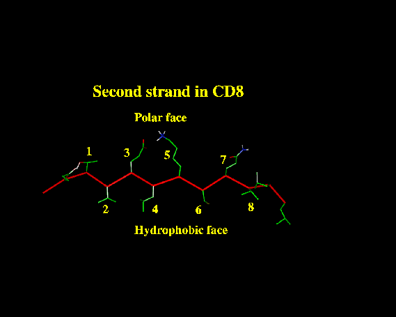
Similarly, the geometry of beta strands means that adjacent residues have their side chains pointing
in oppposite directions. Beta strands that are half buried in the protein core will tend to have
hydrophobic residues at positions i, i+2, i+4, i+8 etc, and polar residues at positions i+1, i+3, i+5, etc.
For example, this beta strand in CD8 shows this classic pattern:
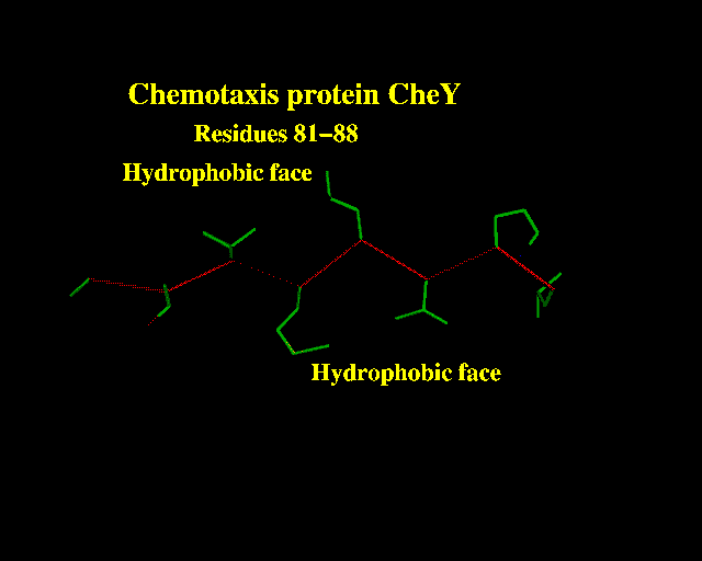
Beta strands that are completely buried (as is often the case in proteins containing both alpha helices and
beta strands) usually contain a run of hydrophobic residues, since both faces are buried in the protein core.
This strand from Chemotaxis protein CheY is a good example:
 The principle behind most manual secondary structure predictions is to look for patterns of residue
conservation that are indicative of secondary structures like those shown above. It has been shown
in numerous successful examples that this strategy often leads to nearly perfect predictions.
The work of Barton et al, Nierman & Krischner, Bazan and Benner & co-workers provide good starting points
for getting doing this sort of work oneself. Some useful references are:
The principle behind most manual secondary structure predictions is to look for patterns of residue
conservation that are indicative of secondary structures like those shown above. It has been shown
in numerous successful examples that this strategy often leads to nearly perfect predictions.
The work of Barton et al, Nierman & Krischner, Bazan and Benner & co-workers provide good starting points
for getting doing this sort of work oneself. Some useful references are:
- Recent reviews on the subject (and on secondary structure prediction generally) See also references therein
- Rost, B., Schneider, R. & Sander, C. (1993), Trends in Biochemical Sciences, 18, 120-123.
- Benner, S. A., Gerloff, D. L. & Jenny, T. F. (1994), Science, 265, 1642-1644.
- Barton, G. J. (1995), Protein Secondary Structure Prediction, Current Opinion in Structural Biology,5, 372-376.
- Russell, R. B. & Sternberg, M. J. E. (1995), Protein Structure Prediction: How Good Are We?, Current Biology, 5, 488-490.
- Some guides for predicting structure:
- Benner, S. A. (1989), Patterns of divergence in homolgous proteins as indicators of tertiary and quaternary structure, Advances in Enzyme Regulation, 31, 219-236.
- Benner, S. A. (1992), Predicting de novo the folded structure of proteins, Current Opinion in Structural Biology, 2, 402-412.
- Some particular examples of protein secondary structure predictions:
- Crawford, I. P., Niermann, T. & Kirschner, K. (1987), Predictions of secondary structure by evolutionary comparison: Application to the alpha subunit of tryptophan synthase, PROTEINS: Structure, Function and Genetics, 1, 118-129.
- Bazan, J. F. (1990), Structural Design and Molecular Evolution of a Cytokine Receptor Superfamily,Proceedings of the National Academy of Science, 87, 6934-6938.
- Benner, S. A. & Gerloff, D. (1990), Patterns of Divergence in Homologous Proteins and tertiary structure. A prediction of the structure of the catalytic domain of protein kinases, Advances in Enzyme Regulation, 31, 121-181.
- Jenny, T. F. & Benner, S. A. (1994) A prediction of the secondary structure of the pleckstrin homology domain, A prediction of the secondary structure of the pleckstrin homology domain, PROTEINS: Structure, Function and Genetics, 20, 1-3.
- Benner, S. A., Badcoe, I., Cohen, M. A. and Gerloff, D. L. (1993) Predicted secondary structure for the src homology 3 domain, Journal of Molecular Biology, 229, 295-305.
- Gerloff, D. L., Jenny, T. F., Knecht, L. J., Gonnet, G.H. & Benner, S. A. (1993), The nitrogenase MoFe protein. A secondary structure prediction. FEBS Letters, 318, 118-124.
- Gerloff, D. L., Chelvanayagam, G. & Benner, S. A. (1995), A predicted consensus structure for the protein-kinase c2 homology (c2h) domain, the repeating unit of synaptotagmin, PROTEINS: Structure, Function and Genetics, 22, 299-310.
- Barton, G. J., Newman, R. H., Freemont, P. F. & Crumpton, M. J. (1991), Amino acid sequence analysis of the annexin super-gene family of proteins, European Journal of Biochemistry, 198, 749-760.
- Russell, R. B., Breed, J. & Barton, G. J., (1992) Conservation analysis and secondary structure prediction of the SH2 family of phosphotyrosine binding domains, FEBS Letters, 304, 15-20.
- Livingstone, C. D. & Barton, G. J. (1994), Secondary structure prediction from multiple sequence data: Blood clotting factor XII and Yersinia protein tyrosine phosphatase, International Journal of Peptide and Protein Research
- Barton, G. J., Barford, D. A. & Cohen, P. T. (1994), European Journal of Biochemsitry, 220, 225-237.
- Perkins, S. J., Smith K. F., Williams, S. C., Haris, P. I., Chapman, D. & Sim, R. B. (1994), The secondary structure of the von Willebrand Factor Type A Domain in Factor B of Human Complement by Fourier Transform Infrared Spectroscopy, Journal of Molecular Biology, 238, 104-119.
- Edwards, Y. J. K. & Perkins, S. J., (1995) The protein fold of the von Willebrand factor type A is predicted to be similar to the open twisted beta-sheet flanked by alpha-helices found in human ras-p21, 358, 283-286.
- Lupas, A., Koster, A. J., Walz, J. & Baumeister, W. (1994) Predicted secondary structure of the 20S proteasome and model structure of the putative peptide channel, FEBS Letters, 354, 45-49.
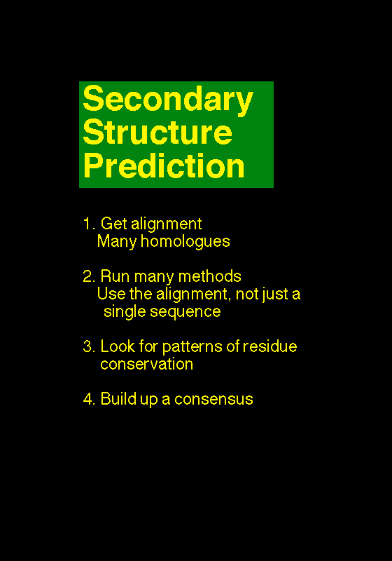
A strategy for secondary structure prediction
In practice, I recommend getting as many state-of-the-art prediction approaches as possible and
combining this with some human insight to give a consensus prediction for the family. If you then align
all of your predictions (including ideas you have based on residue conservation) with your multiple sequence alignment
you can get a consensus picture of the structure. For example, here is part of an alignment
of a family of proteins I looked at recently:
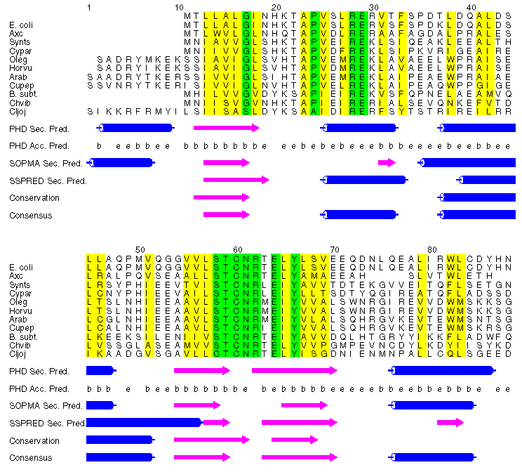 In this figure, three automated secondary structure predictions (PHD, SOPMA and SSPRED) appear below the alignment
of 12 glutamyl tRNA reductase sequences. Positions within the alignment showing a conservation of hydrophobic
side-chain character are shown in yellow, and those showing near total conservation of non-hydrophobic
residues (often indicative of active sites) are coloured green.
In this figure, three automated secondary structure predictions (PHD, SOPMA and SSPRED) appear below the alignment
of 12 glutamyl tRNA reductase sequences. Positions within the alignment showing a conservation of hydrophobic
side-chain character are shown in yellow, and those showing near total conservation of non-hydrophobic
residues (often indicative of active sites) are coloured green.
Predictions of accessibility performed by PHD (PHD Acc. Pred.) are also
shown (b = buried, e = exposed), as is a prediction I performed by looking for patterns indicative of the
three secondary structure types shown above. For example, positions (within the alignment) 38-45 exhibit the
classical amphipathic helix pattern of hydrophobic residue conservation, with positions i, i+3, i+4 and i+7
showing a conservation of hydrophobicity, with intervening positions being mostly polar. Positions 13-16
comprise a short stretch of conserved hydrophobic residues, indicative of a beta-strand, similar to the
example from CheY protein shown above.
By looking for these patterns I built up a prediction of the
secondary structure for most regions of the protein. Note that most methods - automated and manual - agree for
many regions of the alignment.
Given the results of several methods of predicting secondary structure, one can build up a consensus
picture of the secondary structure, such as that shown at the bottom of the alignment above.
Note that you can get predictions like the above (i.e. consensus predictions)
from the very useful JPRED server.
Slides on this subject from my talk:
Slide 5
Slide 6
Slide 7
Slide 8
Slide 9
Slide 10
Slide 11
Slide 12
Next fold recognition.
Back to the Flowchart