Go to the EzMol start page.

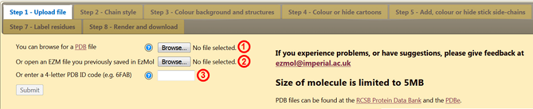
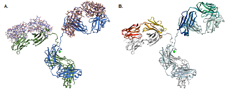
The webpage requires you to upload a file containing the protein structure you wish to visualise. Such files are stored in the Protein Databank (PDB) and are called PDB files. The PDB and PDB files are discussed in the Teaching Portal. You can (1) upload a PDB file from your computer, (2) upload an EZM file containing a previous EzMol session or (3) use a unique PDB ID code to retrieve a PDB file from the databank. The figures in this activity were generated using the antibody (an immunoglobulin G2a) in PDB 1IGT.

Antibodies

The protein used as an example here is an antibody, a protein that recognises foreign elements in our bodies. The RCSB PDB published a short introduction to antibodies and their structure as part of its Molecule of the Month, available here.

Moving the protein

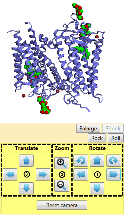
On the left of the screen is a white square containing the protein (Figure 2). As you explore EzMol, this square will remain present and allow you to visualise the protein. You can rotate the protein by left-clicking and dragging it within the visualiser, or by using the options in square (1) (right panel). You can zoom in and out using the right click (and dragging the protein) or square (2) (middle panel) and you can drag the protein by clicking with the wheel of the mouse or square (3) (left panel).

You can turn on and off a rocking or rolling motion by clicking the corresponding buttons. The ‘Enlarge’ and ‘Shrink’ buttons change the size of the visualiser. You can always go back to the default view by clicking ‘Reset camera’.

EzMol provides you with some information about the structure you are viewing, including the name of the structure, its PDB ID and the date it was deposited into the PDB.

The tab ‘More details’ provides you with extra information, including the number of chains and residues, the organism the molecule is from, the experimental techniques used to solve the structure, the resolution, the molecular weight of the molecule and the people who published the structure.

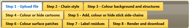
To move to the other steps in the EzMol workflow, use the top navigation bar shown in Figure 3 below.

In the top navigation bar, click on ‘Step 2 - Chain style’. You can change the style of each chain separately.

The cartoon display only shows the backbone of the protein (and not the side chain atoms) according to secondary structure.

The stick display, on the other hand, shows the bonds between all atoms other than hydrogen in the molecule (including side chain atoms). Tick ‘Colour stick heteroatoms by element’ to show different atoms with different colours. This allows easy identification of the atoms making up biological molecules.

Chains can be specifically hidden, allowing the visualisation of only part of the molecule. Each chain can also be displayed as a surface, which shows the space occupied by the molecule.

You can change the background colour. When saving and printing a view of a protein (cf. Step 8), it is traditionally advised to use a white background.

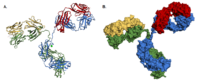
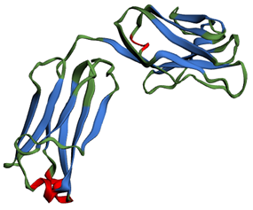
You can colour the cartoon representation, the sticks and the surface of each chain. This is a particularly useful way of conveying information about the different polypeptide chains constituting a protein, as shown in Figure 4 below.

If a chain is displayed as sticks with heteroatoms coloured according to element, changing the colour of the stick representation in this tab will only affect the carbon atoms, as shown in Figure 5A.

You can also use the ‘Advanced: Cartoon gradients’ tab to colour the protein with a colour gradient, using either a predefined one (drop-down menu in the ‘Preset gradients’ column) or making your own (by defining the start and end colours as well as the gradient path). Some of the preset gradients are shown in Figure 5B.

Colouring individual residues

You can select a colour from the drop-down menu and then select the residues you wish to display in that colour. You can also choose to hide residues by selecting the eraser and then selecting the appropriate residues.

Secondary structure elements

By clicking on ‘Apply by secondary structure type’, you can choose to colour specifically all residues in α-helices, β-strands or coils, as shown in Figure 6. Teaching resources about protein secondary structure are available in the Teaching Portal.

Side chain properties

The ‘Apply by chemical type’ tab allows you to colour the cartoons according to the properties of their constituting amino acid residues.

Non-polar and aromatic side chains (R groups of the amino acid residues) are hydrophobic: they do not interact with water and tend to cluster away from it. Polar and charged (either positive or negative) side chains, on the other hand, are hydrophilic: they readily interact with water.

You can select a colour and then select specific amino acid residues to display their side chains as sticks (of the colour you have selected). You can select the eraser and then select specific amino acid residues to hide their side chains.

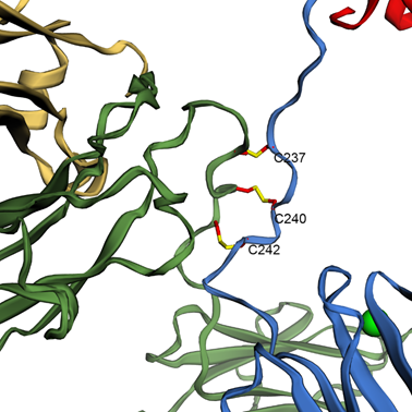
This is useful as the relative position of two side chains (or a side chain and the backbone, for instance) is sometimes functionally relevant, e.g. to form a salt bridge between residues. Figure 7 shows how three disulphide bonds can be shown in the antibody from PDB 1IGT.

You can select a colour and then select specific residues whose surface you would like to highlight. If the protein was already shown as a surface, then the patches corresponding to the residues you have selected will simply adopt the chosen colour. However, if the protein was originally displayed as a ribbon or sticks (which you can change in ‘Step 2 - Chain style’), then a transparent surface will be generated for the entire protein but only the selected residues will be coloured.

Click on ‘Apply by scheme’. You can colour the surface according to one of three characteristics: the temperature factor (B-factor), hydrophobiity and charge. The B-factor is a measure of how flexible an atom is in the structure. A high B-factor indicates that the atom moves a lot, whereas a low B-factor shows that it is fixed in space.

You can also set the colour scheme. If one chain was hidden, it will appear when you select one of the three schemes, you can hide it again by going back to ‘Step 2 - Chain style’ and unclicking ‘Display surface’ for that chain.

This tab allows you to label the amino acid residues in the protein. There are several options for the type of label you want to display and you can change the colour of the text (foreground) and the label background. You can choose to remove the label background by making it transparent (last square in the colour menu).

To select which residues to label, click ‘Apply to individual residues’. Labelling important residues is very useful to produce informative figures, which you can save as explained below (‘Step 8 - Render and download’).

At any point during your work, you can click on ‘Step 8 - Render and download’ (in the top navigation bar) and then ‘Click here to save the image’. This will save a PNG file of the view currently displayed in the visualiser.

You can also click on ‘Save your work log’ to download an EZM file containing the changes you have made during your session (e.g. changing the display style or the colour of the protein). You can then load that file later as described in Step 1.